Join Dennis Taylor for an in-depth discussion in this video, Sort by background color or font color, part of Excel 2016 for the Mac: Managing and Analyzing Data. In Excel 2003 and 2002 for Windows or Excel 2008 and 2004 for Mac, follow these steps. Select all of the cells that you want to sort by alphabetizing two or more lists in the range. Select Data on the toolbar and choose Sort.

Autofilter is one of the most powerful features of Excel if you need to work with data in tabulated (table) format. It lets you treat a range of cells as a table and then filter out certain rows based on different criteria. It is very powerful if you need to 'mine' data in a list and find out specific information about the data in that list. This tutorial covers how to set up a data table in Excel to use with Autofilter, and also shows you how to enable Autofilter and use it for basic filtering. This lesson is applicable for all versions of Excel (including Excel for Mac) although the visual presentation of the options may change from version to version.

Prepare your data for Autofilter To use Autofilter, first ensure you have a table of data to work with. Follow these simple steps to check that your data table is ready to use with Autofilter: • Check that your data is organised in columns. Each column should have a heading that explains what sort of data is in the column. • Your column headings should occupy just one row of the spreadsheet, as shown in this example: ​ • You should avoid using column headings in two rows, as shown in the following example, because they can confuse Excel's Autofilter feature and stop it working as it should.

While you can still use Autofilter if you have headings in two rows as shown here, it's much easier if you stick to headings in just one row: • Next, make sure there are no empty columns or rows in your data. Excel is good at sensing the start and end of a data table by looking for empty rows and columns, and will ignore data after an empty row or column. • A quick tip to check if your data is formatted in one contiguous range (a fancy way of saying 'one block of data', which is used a lot in the Excel world) is to click a single cell in the table then press CTRL+* (or CTRL+SHIFT+8 if you don't have a separate number keypad). This automatically selects the whole table. You'll then see if you have any problems with the layout of your table. • This example shows a table that is in a contiguous range: • This table has an empty row; after pressing CTRL+* to select the table, you can see that the rows after the empty column have been ignored: • Similarly, this table has an empty column, so the columns to the right of the empty column have been ignored: • • Note that empty cells within the table are OK. What isn't OK is a whole row or a whole column of empty cells.

The CCleaner tool for Mac OS Sierra is a freeware program which works like a privacy, optimization and cleaning tool all at once. It is used for removing the unwanted files from the computer system. It helps Mac to perform faster by cleaning up the disk space. CCleaner ® for Mac CCleaner is the number-one tool for cleaning your Mac. It protects your privacy and makes your Mac faster and more secure! Download Free Version Buy Now. Faster Computer. A Mac collects junk and unused files just like a PC. Find and remove these files with the click of a button so your Mac can run faster. Is there a date for an macOS Sierra compatible update available? I just updated my iMac and recognized that, beside some other tools too, ccleaner doesn't s. CCleaner for Mac scans your system to remove all kinds of files that can slow your Mac down and then removes the items you want. Through this app's intuitive. Added macOS Sierra Beta. The Piriform team are happy to announce the latest release of CCleaner for Mac. CCleaner Mac v1.14 brings updated browser cleaning along with macOS Sierra Beta support! A list of changes can be found in the change log below.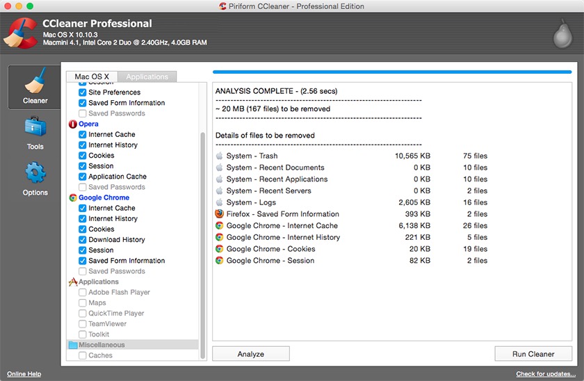

• Finally, check that you have consistent data types in all cells. • For example, if you have a date column, make sure all the values in that column are dates (or blank). • If you have a quantity column, make sure all the values are numbers (or blank) and not words. • This is not a hard and fast rule, but it will make it much easier to use the features of Autofilter if you follow them wherever possbile. At this point, if everything is looking OK, you're ready to move on to the next step. Enable Autofilter Once your data range that meets the criteria above, you are ready to apply the Autofilter feature: • Select a cell in the range. • Any cell will do, but make sure you don't select more than one cell or Excel will apply the Autofilter to the selected cells rather than the whole table.

• You may prefer to select all of the cells in the data range if you want - this is a good idea if you have columns with headings in two or more rows (as discussed above). • Next, click the Sort and Autofilter button on the Home tab of the Excel ribbon toolbar, then click Filter. • The first row in the table (the header row) should change, with a small drop-down arrow on each cell in the header row, similar to the example below: ​ You are now ready to start using Excel's Autofilter feature. Using Excel's Autofilter feature to filter your list You can now filter the table based on the values in the table by clicking the buttons to the right of the column heading. This will show a drop-down list as shown here: In this example, we've clicked the Autofilter button for the Salesperson. Based on the selection we have made, the list will be filtered to show only rows where Mike is the Salesperson. Other options you have here will allow the following: • Sorting by Salesperson.